Once upon a time I was replicating the UMAP of the gene expression profiling (L1000) of 1,327 small molecules perturbation from the Drug Repurposing Hub (Way et al. 2022). To my surprise, the first UMAP I generated was seriously odd. I still don’t have a clear explanation of what went wrong but I am sharing my exploration of the issue in case someone comes accross it. A here be dragons tale of computers doing unexpected things which affect analysis.
Preamble
Skip if you are familiar with dimensionality reduction or L1000 gene expression profiling.
Dimensionality reduction
This is not a statistiscs post so I will not deep-dive into UMAP or PCA, but here is a short overview for those new to dimensionality reduction to get a bit of background.
In Omics and other data modalities, we often have to make sense of multi-dimensional data: many samples (ideally) and many features. Unfortunately, humans can’t make sense of more 3-4 feature dimensions, and forget about plotting to visualize high-dimension space. So a common strategy undertand high-level multi-dimensional data is what is called dimensionality reduction. This projects the existing features in a new loew dimentions space which still capture local clusters and the global structure. It then allows us to plot these new dimensions which capture most, or at least a good portion, of the information in the data.
The most well know of these methods is perhaps PCA, with UMAP and t-SNE coming to fore in recent years. PCA is a linear method focusing on global variance (big picture), faster, interpretable, good for feature extraction / reduction; whereas UMAP is non-linear and better at revealing local clusters and complex structures has been slowly replaving t-SNE, at least in my domain (genomics).
A neat little trick is to run PCA on the data, take top N compoments to run UMAP thus reducing computation time. This trick is frquentely used in single-cell RNAseq, and also used the analysis I was tryign to reproduce. The PCA will sort of clean the data by reducing the co-linarity, keeping the local sructure intact.
L1000 perturbation profiling
This is also not a post about the biology of the experimental methodology but tldr; L1000 is a gene expression profiling method (not sequencing based) which captures the expression of 1000 “landmark” genes, and uses this information to predict the expression of aprox. another 14.000 genes.
In the paper I am referring to, it was used along Cell Painting, which uses a set of subcell markers to captures cell morphological changes, to profile how compounds in the Drug Repurposing Hub affect gene expression and cell morphology. Neat paper.
Original analysis
My initial goal to use published data for a simple analysis. Been there, done that. As per usual, and after downloading the data wanted to run a quick sanity check - could I reproduce the UMAP figure (2A) for the LINCS data? It lead me into a rabit hole.
I started using the existing code that the authors provided for data processing in python. This reads the data, runs the PCA, selects the top 200 components, and creates the final embedding with UMAP - fairly standard as mentioned above.
I did make a seemingly harmless change: instead of running umap in python, I took the PCA components and creates the UMAP embeddings in R. This is possible using the reticulate package - because the past, present and future of data science is polyglot. I was basically using this small analysis to POC reticulate and run UMAP in R.
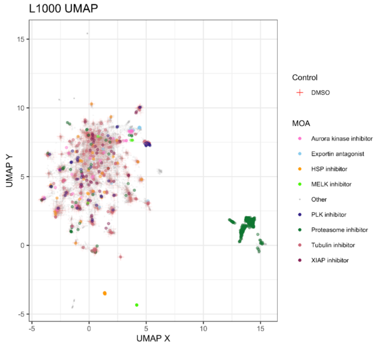
Regardless, the expection is that I should be getting a good aproximation of this plot:
It show a failry dense aglomeration of points which include all the DMSO controls, and a proeminant group of data points (right) which seems to be composed of nearly al the Proteosome inhibitors.
Let’s how the replication comes along.
Prepare data
Let’s call all necessary R libraries:
Code
Sys.setenv(RETICULATE_PYTHON_ENV = here::here("posts/2025-11-25-ump-r-python/.venv")) ## I can't have nice thingslibrary("reticulate")library("umap")library("dplyr")library("data.table")library("ggplot2")library("magrittr")library("tictoc")theme_set(theme_light())#reticulate::py_config()## reticulate::repl_python()
Followed by the python code to:
read data in
perform PCA and
extract the top 200 components
Code
import pathlibimport numpy as npimport pandas as pdimport umapfrom sklearn.decomposition import PCAimport plotnine as plimport time## Load L1000 profilesstart_time = time.time()file="https://github.com/broadinstitute/lincs-profiling-complementarity/raw/5091585bde14c33d6819fa6b494e352a064fbeb4/1.Data-exploration/Profiles_level4/L1000/L1000_lvl4_cpd_replicate_datasets/L1000_level4_cpd_replicates.csv.gz"df = pd.read_csv(file, low_memory=False)print("--- Data reading: %s seconds ---"% (time.time() - start_time))
--- Data reading: 10.993651151657104 seconds ---
Code
features = df.columns[df.columns.str.endswith("at")].tolist()meta_features = df.drop(features, axis="columns").columns.tolist()features_df = df.loc[:, meta_features]data_df = df.loc[:, features]## Transform PCA to top 200 componentsn_components =200pca = PCA(n_components=n_components)pca_df = pca.fit_transform(data_df)pca_df = pd.DataFrame(pca_df)pca_df.columns = [f"PCA_{x}"for x inrange(0, n_components)]print(pca_df.shape)
(27837, 200)
We move the PCA compoments to R and tidy the Mechanism of Action (MOA) annotations by keeping only the most the 10 frequent and lumping the the rest together. This is purely for visualization purposes.
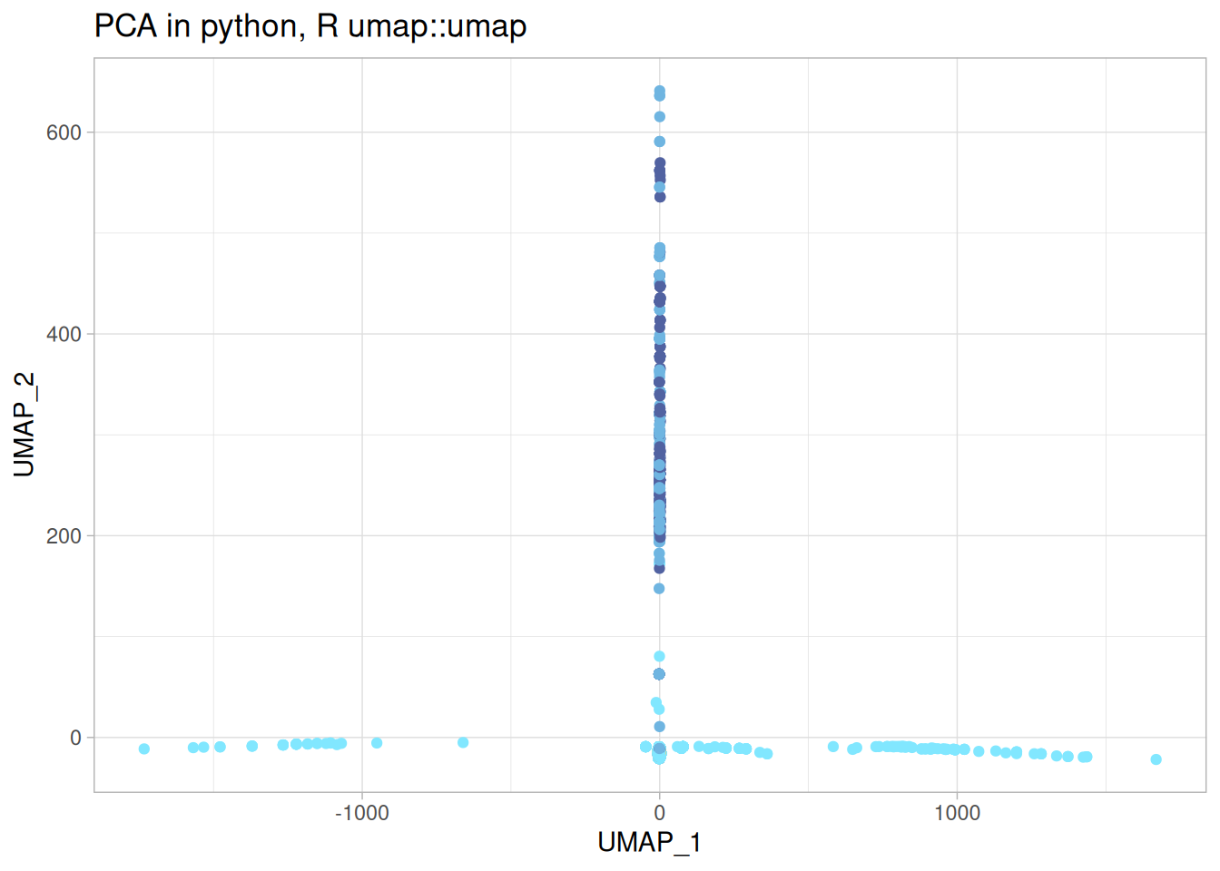
umap_r_p <-cbind( umap_r$layout, features_df) %>%rename("UMAP_1"=1,"UMAP_2"=2 ) %>%ggplot(aes(x = UMAP_1, y = UMAP_2, color = moa)) +geom_point() + khroma::scale_colour_managua(discrete =TRUE) +labs(title ="PCA in python, R umap::umap" ) +theme(legend.position ="none")umap_r_p
Oh my.
This is wild! I used the same parameters as provided in the original umap code, and even accounting for different implementations having different aproximations, or different random seeds, it shouldn’t be this different. Not only is the shape and the relative location of the data points quite different, but so is the range of the UMAP embeddings. Something is off.
Note
Issues with UMAP giving our wildly different results even if the analysis is done stricly in python are not new. Here someone reports how a diferent version of numba, a library that umap-learn relies on to optimize execution speed, caused massive differences:
https://github.com/lmcinnes/umap/issues/1232
so this is not an R thing, it’s computers thing.
So what is going on?
umap-learn via {umap} in R
Could this be the R “native” implementation?
Note
It’s actually using {Rcpp} in the background to call c++.
Thankfully the {umap} package also provides a argument to call the python {umap-learn} - yeah, I know, it’s turtles all the way down - which allows to test the call to {umap-learn}:
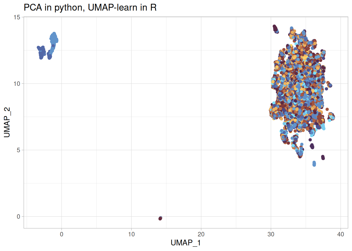
umap_learn_r_p <-cbind( umap_learn_r$layout, py$features_df) %>%rename("UMAP_1"=1,"UMAP_2"=2 ) %>%ggplot(aes(x = UMAP_1, y = UMAP_2, color = moa)) +geom_point() + khroma::scale_colour_managua(discrete =TRUE) +labs(title ="PCA in python, UMAP-learn in R" ) +theme(legend.position ="none")umap_learn_r_p
Note
Note how much faster the python code is - it has been optimized with some compile on run magic which to my surprise beats the R/c++ implementation.
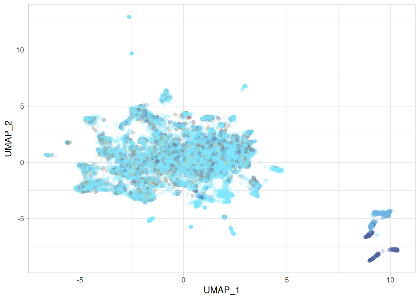
Using {umap-learn} from python, note the argument method = "umap-learn", gives a more sensible looking embedding. Not quite the same as the paper, but anyone who tried to replicate papers know that stuff happens.
But António, I hear you say at the back, in the paper they did the umap purely in python.
Fine.
You are correct but I counter that the method implementation in any given language shouldn’t affect the main conclusions so much.
UMAP in python
But I will humor you and do the thing in python only.
/home/adomingues/Documents/projects/datalyst/posts/2025-11-25-ump-r-python/.venv/lib/python3.12/site-packages/umap/umap_.py:1952: UserWarning: n_jobs value 1 overridden to 1 by setting random_state. Use no seed for parallelism.
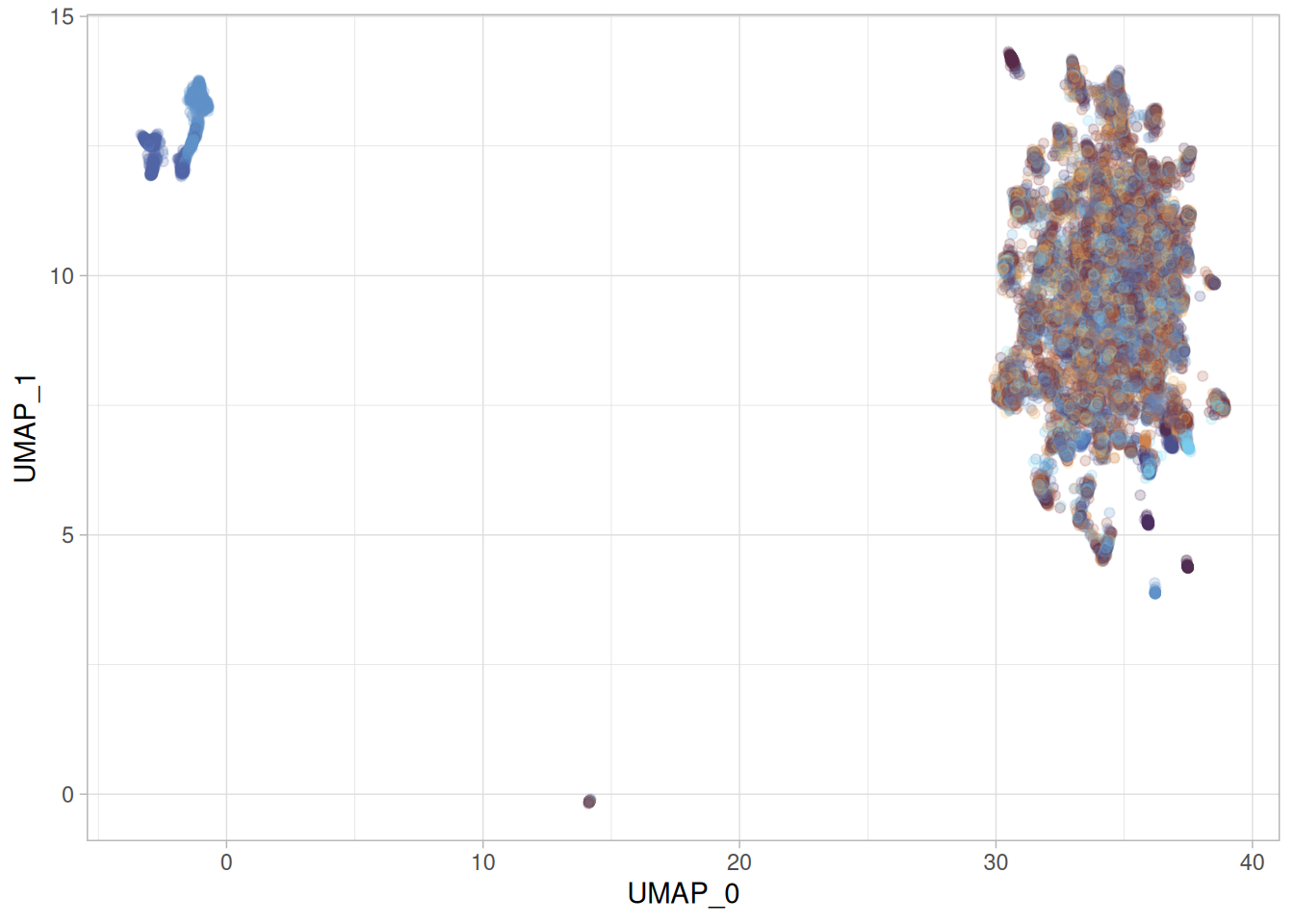
py$full_umap_embedding_df %>%ggplot(aes(x = UMAP_0, y = UMAP_1, color = moa)) +geom_point(alpha =0.2) + khroma::scale_colour_managua(discrete =TRUE) +theme(legend.position ="none")
That is pretty much the same as the one we obtained by calling umap-learn from R. So the python umap-learn is reproducible.
At this point, what I am thinking is that reticulate is somehow messing my environment, linking different c++ libraries (?) and thus affecting the R/c++ implementation.
uwot test
There is another R implementation of UMAP implemented in the packaged {uwot}, which also calls c++ via Rcpp. Is this also affected?
Code
library("uwot")
Loading required package: Matrix
Attaching package: 'uwot'
The following object is masked from 'package:umap':

    umap
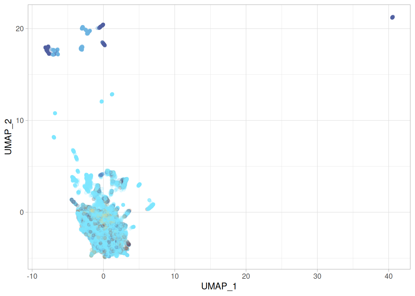
The second thing, and most important, is that whilst the result is not the same as umap-learn is sensible enough that we could optimize the hypermaraters to get it closer.
Warning
Note that thre is no single “correct” umap representation. By changing parameters we will obtain different embeddings which will represent different aspects of the data.
I refer to his blog which demonstrates this point quite well: https://jef.works/blog/2022/01/19/exploring-umap-parameters/
But it doesn’t completely support or disprove my hypothesis that it’s something to do with the c++ libraries. It does seem like it isn’t an issue with c++ because we don’t have an extreme result like in umap::umap, however {umap} and {uwot} use different libraries, so who knows. I certainly don’t know enough c++ or what mumba is doing for umap-learn to determine how important this is.
The big reveal
(not that big or much of a reveal - more of a damp squib)
During all of this testing and messing about with R / python and writing bug reports there was this one time when umap::umap resulted in a resonable plot. I had a hard time reproducing it, but just before posting this I thought to myself:
what if I clean up the R session by remove all libraries / objects and unset the reticulate env variables and do the entire analysis in R?
library("umap")library("dplyr")library("data.table")library("ggplot2")library("magrittr")library("tictoc")theme_set(theme_light())tic()## data prepl1000 <-fread("https://github.com/broadinstitute/lincs-profiling-complementarity/raw/5091585bde14c33d6819fa6b494e352a064fbeb4/1.Data-exploration/Profiles_level4/L1000/L1000_lvl4_cpd_replicate_datasets/L1000_level4_cpd_replicates.csv.gz") %>%as.data.frame()toc()