This post are my notes on how to use a very large genomics dataset in a under-resourced computer - using TileDB and a combination of python and R. I have been interested in TileDB for a while but I never had opportunity to use it at work. Luckily, one of my many personal projects involves querying a very large data set (LINCS 2020, 115 GB data) which doesn’t fit in memory, and thus is perfect to give tiledb a proper go. This might be useful for folks working with larger than memory data, specially single-cell data.
There are many other ways this data could be represented on-disk and still be performant. I picked TileDB mostly because I can use the existing SomaAPI, which was built for single-cell data but could be extended for other gene expression data.
Note
If you have single-cell data in anndata format, most of the data transformations being done in this post are not necessary and you can skip straight to Section 5.4.
There is a lot of rambling and concepts being explained in this post, not all necessary to understand the technical bits, so here is a diagram of what I will be doing:
Code
---config: look: handDrawn theme: forest---flowchart LRsubgraph h5 is out-of-memory and BioC friendly A[GTX] --> |Gene expression| B[h5]end D[csv] --> |Gene and Experiment metadata| Csubgraph anndata has chunked ingestion to TileDB B --> C(SingleCellExperiment) C --> E(anndata) E --> F[(TileDB-SOMA)]end
---
config:
  look: handDrawn
  theme: forest
---

flowchart LR
subgraph h5 is out-of-memory and BioC friendly
    A[GTX] --> |Gene expression| B[h5]
end
    D[csv] --> |Gene and Experiment metadata| C

subgraph anndata has chunked ingestion to TileDB
    B --> C(SingleCellExperiment)
    C --> E(anndata)
    E --> F[(TileDB-SOMA)]
end
Diagram of how data will be moved between formats to finally get it into the DB. Only necessary to keep memory use as low as possible.
Biological motivation
LINCS2 is a pretty unique dataset consisting of millions of chemical and genetic perturbations in multiple (cancer) cell lines (see Section 3.1). The chemical perturbation signatures have reportedly been used extensively for drug re-purposing, mechanism of action (MoA) identification, and model training. However, the genetic perturbation data is less recent and has (i) not been as used, and (ii) is not so well characterized.
From a data science / computational biology perspective, and in my view, the genetic perturbations have one key advantage:
There is a very clear ground truth - if a gene is knocked out, the expression of that gene should go down.
This means that if one were to create a model to predict the effect of a gene perturbation, the validation is quite straightforward. For chemical perturbations the situation is far more complex and making predictions is harder:
Not all compounds have a known target protein
Some compounds might have multiple targets owing to:
The target is a protein complex
Polypharmacology
Off-target effects
The MoA of a compound is not know (or is poorly annotated)
The pathways affected by the compound is not now.
So whilst the chemical perturbations are very useful for Drug Discovery and Development, I have some doubts about how good the modelling of those can be.
But there is a catch: this is a very large large dataset (by the standards of gene expression data). At 115 GB for the matrix alone (3,026,460 x 12,328), excluding the perturbation metadata - a measly 643.81 MB - this too large for a regular laptop to handle in memory. So how to use this data in the most computationally efficient manner?
Computational solution
TileDB-SOMA with it’s out-of-memory capabilities to facilitate data querying, and potentially ML, seems like a good solution. This pretty important because I will be using a dataset of 115 GB in size to make a DB and perform queries on a 16GB RAM laptop. Normally this would require loading the data into memory but I will show it doesn’t have to be that way.
In addition, it implements the CZI data standard for single cell data (soma) which means I could leverage this API for some the work.
Not that his is super relevant, but the laptop is running Ubuntu server edition, which means that those 16GB stretch more than if one was running a Desktop edition. The GUI (Gnome) takes away quite a bit of memory.
I will again use a mix of R - to take advantage of existing and mature genomics packages - and python because the TileDB-SOMA API is slightly more mature.
Some concepts
LINCS2
What is LINCS2? It’s a data set of the gene expression obtained after different perturbations:
It was generated in many cell lines
Includes chemical (small molecules) and genetic perturbations perturbations (CRISPR, shRNAs, but also over-expression)
The data came out in several iterations, with LINCS 2020 being the final release.
This is a pretty comprehensive data set:
The LINCS 2020 beta release data set contains 1.2 million signatures with 720,216 compound treatment GESs of 34,418 compounds, 34,171 gene over-expression on 4,040 genes, 318,208 gene knockdowns on 7,976 genes using shRNAs on 4,917 genes (177263) and CRISPR on 5,158 genes (140945). Out of 720,216 compound treatments, it includes 34,418 drug-like small molecules tested on 230 different cell lines at multiple concentrations and treatment times. To minimize redundancy of perturbagens having many signatures in different cell lines, dosage and treatment times, the ‘exemplar’ signature for each perturbagen in selected cell lines was assembled. These signatures are annotated from CLUE group and are generally picked based on TAS (Transcriptional Activity Score), such that the signature with the highest TAS is chosen as exemplar. The generated LINCS2 dataset contains moderated z-scores from DE analysis of 12,328 genes from 30,456 compound treatments of 58 cell lines corresponding to a total of 136,460 signatures. It is exactly the same as the reference database used for the Query Tool in CLUE website. Like the LINCS database, users have the option to assemble any custom collection from the original LINCS 2020 beta release dataset. source
L1000
What should also be noted is that the LINCS data is not an genome-wide gene expression survey. The method used is a bead-hybridization assay in which only 978 genes are directly measure - thus L1000 (I allow the creative license for the rounding up). The authors demonstrated that 1000 genes where enough to create a model which captured nearly all gene expression variation and could be used to estimate (predict) the expression another 11,350 genes (see).
Why only measure 1000 genes instead using RNA-seq?
This makes the method extremely cheap vs conventional sequencing. At the time Perturb-seq had just been published, and DRUG-seq (which I quite like!) was not a thing. We have to take in mind that this dataset is made of ~3 million data point (a well with treated cells). At a very generous estimate of €50 per data point for a DRUG-seq type sequencing run, that’s about 1 million euros total. And that excludes any other costs associated with the experiments (staff, reagents, instrumentation). It’s a lot, so L1000 at around €2 per data point starts looking like a good deal.
The price advantage of L1000 was not enough for the method to take off, and to the best of my knowledge it hasn’t been used outside of LINCS and similar projects. Besides only measuring ~1000 genes, which need to be well expressed, another disadvantage) is that readout is noisier than sequencing. With decreasing prices of sequencing, an novel single-cell perturbation methodologies coming into the space the price advantage became less important.
The LINCS dataset set itself is still pretty unique though.
CMAP
CMAP stands for connectivity map and is the database of non-redundant perturbation signatures, one per per compound / RNAi per cell lines, and allows researchers to match their own signatures to the database. A typical use case would be:
A gene expression signature for a compound of unknown activity was obtained and using CMAP it can be used to match existing signatures. The closest matches will give clues as to what is the most likely MoA, class of compounds, or gene/proteins target. At least in theory. In practice the query results tend to be quite messy and requiring a lot of cleaning up before one can gain any meaningful insights - at least in my experience.
Note
A gene signature is basically a ranked list of up and down-regulated genes. The are a number of methods (similarity metrics) which can be used to retrieve the best matches - quite a few them implemented in signatureSearch. The method used in LINCS is a variation of the Kolmogorov-Smirnov enrichment statistic (ES). These methods tend to be computationally slow.
LINCS2 in TileDB: why?
As I mentioned, I have a small project in the works that will use this datasets. Whilst there is a package, signatureSearchData, that contains most of the LINCS2020 data and wrapper code to query it, sadly it is not a viable option for me:
I am interested in the genetic perturbations which are not part of the provided DB;
Whilst signatureSearchData provides instructions to create new DBs for the genetic perturbations, the data is loaded into memory and I only have 16GB RAM available.
Note
Yes I could use a “cheap” AWS instance or whatever, but I would need something like a r8g.8xlarge instance (256 GB RAM), which is fairly expensive for a personal budget. Secondly, if you ever worked with AWS, cheap or simple are not words you would associate with it.
TileDB, and specially their SOMA data model serves my purposes quite well. TileDB is an unusual but powerful proposition in data as it has DB on it’s name, but it’s less a database and more a way to structuring and connecting different data modalities. It’s also the name of company behind the tech. Their blurb is:
TileDB is foundational software designed by scientists for scientific discovery. TileDB structures all data types, including data that does not easily fit into relational databases. Built on a powerful shape-shifting array database, TileDB handles the complexities of non-traditional “unstructured” multimodal data, such as genomic variants, bulk and single-cell transcriptomics, proteomics, biomedical imaging, as well as the frontier data of the future.
Has libraries/functions to make single-cell data analysis quite straightforward
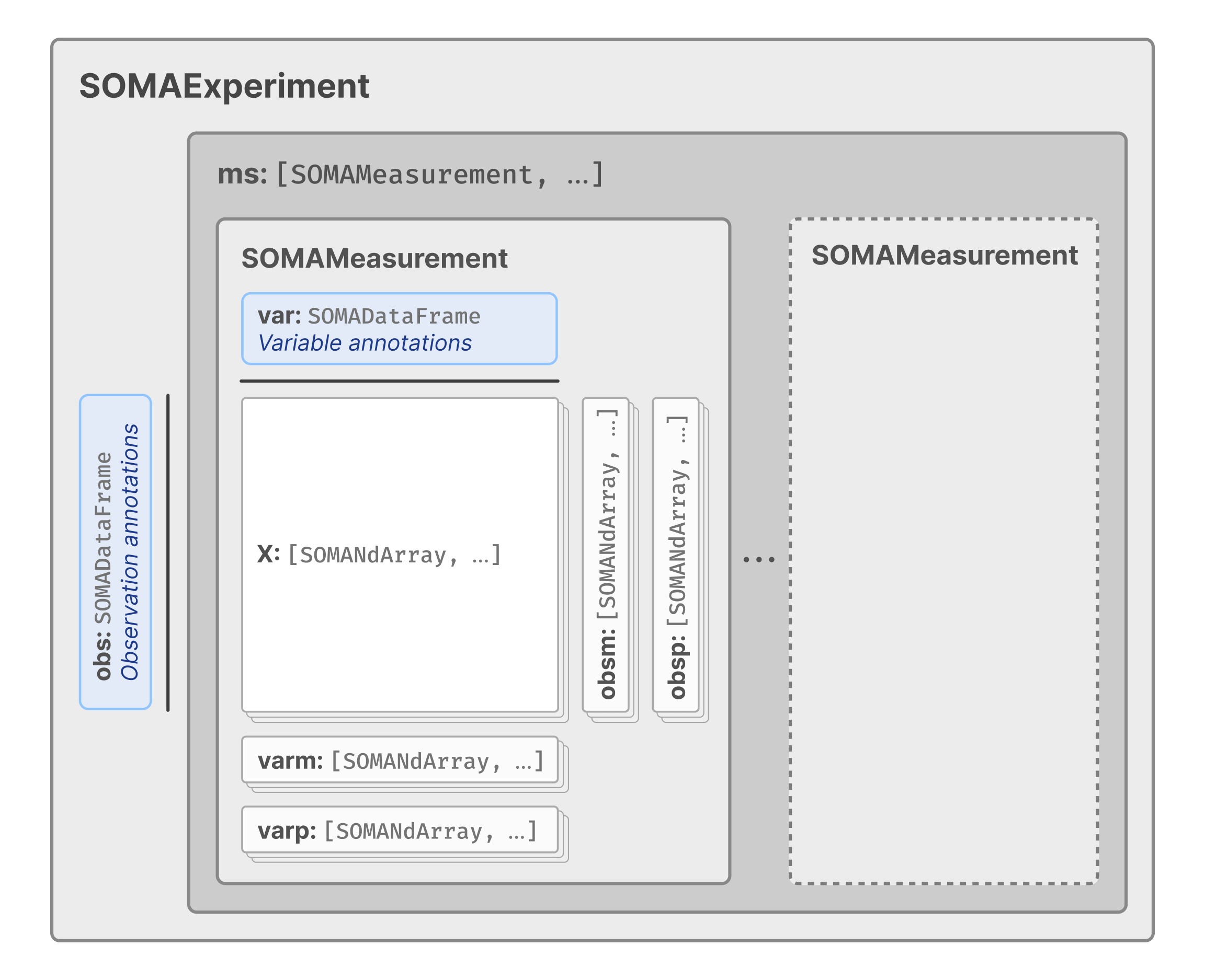
This last part caught my eye because this means that in principle any gene expression like dataset that can be fitted into an anndata or SingleCellExperiment would leverage existing APIs - removing the need to write a lot of new (redundant) code. If you look carefully the data spec looks very much like that of Biocondutor’s singleCellExperiment (itself an extension of SummarizedExperiment):
Data model for TileDB-SOMA
And it turns out that the LINCS data format, GCTx which is based on HDF5, but is also conceptually similar to singleCellExperiment and by extension to Tile-db soma. This means that I could use a series to data format conversations, using existing tools, to obtain a DB which allows out-of-memory querying.
Yay for the many redundant data formats in bioinformatics.
Create TileDB
Some good folks were kind enough to wrap the data in a R / bioconductorSummarizedExperiment object with an delayed array back end. And this important because it reduces the need to load data into memory. However, this object doesn’t include all perturbations - the genetic perturbations are missing, specially those released in 2020 and corresponding to largest set.
Another reason why I can use this existing signatureSearchData dataset is that only level 5 data is included. These are single vectors of gene expression, one per perturbagen and per cell line - meaning that replicate values, or multiple concentrations in the case of compound perturbations, are not longer included. This is fine for biological exploration, but not for QC and data exploration. My database will be on level 4 data which includes differential expression for individual replicates vs the plate median. I want that granularity.
So how to build the tiledbsoma from the raw data (h5 and plain text files)? Since I was not keen on re-inventing the wheel, I though I could make use of the tutorial provided in the vignette to make a SummarizedExperiment and then convert it to
Basically:
gtx -> h5 -> singleCellExperiment -> tiledbsoma
The critical aspect is the conversion to h5 which will allow out of memory operations.
1. Data download and prep
The data is stored in GEO, but the most convenient location are the S3 download links provided by clue.io:
Before we can start any format conversion, there is of course some data cleaning involved. I’ve learned the hard way that to create level 4 databases, and possibly level 3, we need to obtains the column names from the gtcx file - otherwise It’s a mess.
The data preparation step consists of collecting the row (sample) and column ids (genes) to ingest later. This is necessary to avoid issues data points which are present in the full sample metadata table but not in present in the matrix for a particular data level - missing data due to not passing QC for example.
The column names are also formatted to make them computer-friendly - another one of those things that will cause headaches in the future if note done upfront.
This is ok but only contains the matrix with the expression values, and column row names. Not of much use as is. So I’ll need to add some information about the perturbations (and the genes).
Now the sce object has the assay data (gene expression matrix), colData (perturbation metadata) and rowData (gene IDs), we can finally save it has an anndataobject. This is basically python’s version of the singleCellExperiment object but it’s supported by TielDB-SOMA for chunk ingestion (goes nice on the memory):
Anndata object diagram
One would expect that chunked ingestion would also be possible with singleCellExperiment but the API is lagging behind:
However, the Python API does support chunked-ingests of H5AD files via AnnData’s “backed mode.” This means the data from the .X matrix is streamed directly from the H5AD file into the SOMA array on disk, without loading the entire matrix into RAM. https://github.com/single-cell-data/TileDB-SOMA/issues/4291#issuecomment-3434169342
So let’s do that extra step and save the anndatah5ad :
# A tibble: 6 × 33
  soma_joinid obs_id bead_batch nearest_dose pert_dose pert_dose_unit pert_idose
        <int> <chr>  <fct>             <dbl>     <dbl> <fct>          <fct>
1           0 ABY00… b15                  NA        NA ""             ""
2           1 ABY00… b15                  NA        NA ""             ""
3           2 ABY00… b15                  NA        NA ""             ""
4           3 ABY00… b15                  NA        NA ""             ""
5           4 ABY00… b15                  NA        NA ""             ""
6           5 ABY00… b15                  NA        NA ""             ""
# ℹ 26 more variables: pert_time <dbl>, pert_itime <fct>, pert_time_unit <fct>,
#   cell_mfc_name <fct>, pert_mfc_id <chr>, det_plate <fct>, det_well <fct>,
#   rna_plate <fct>, rna_well <fct>, count_mean <int>, count_cv <int>,
#   qc_f_logp <dbl>, qc_iqr <dbl>, qc_slope <int>, pert_id <chr>,
#   sample_id <chr>, pert_type <fct>, cell_iname <fct>, qc_pass <int>,
#   dyn_range <dbl>, inv_level_10 <dbl>, build_name <lgl>, failure_mode <fct>,
#   project_code <fct>, cmap_name <chr>, new_id <chr>
Code
toc()
6.229 sec elapsed
Now let’s get some expression data for a subset of the array:
Code
tic()## format is interesting with columns for X, Y and data. Not a rectangular format as we would expectexperiment$ms$get("level_4")$X$get("data")$read(coords =list(0:10L, 0:10L))$tables()$concat()$to_data_frame() %>% tibble::as_tibble()
What we would normally want to do though is to filter the data data with a combination of perturbations and / or obtain the expression of certain genes. Here I was asking for the expression values of GRIN1 and GRIN2B in a all the genetic perturbations of GRIN1 that pass experimental QC:
The main one is that doing these operations, mostly on-disk, is very slow. Each of these transformations takes several hours to a day. This is not unexpected because are talking about > 100GB of data begin passed around in a fairly low end system.
This comes to the second point: it uses a lot of disk space. As far as I can tell none of these data formats, including TileDB does any meaningful compression, so using a 500GB disk was not enough and I had to use a mounted remote disk. It is in my home network, but it still impacts speed massively.
Comments
I welcome any comments or suggestions at amjdomingues at gmail.com or ping me on Linkedin / Mastodon


Comments
I welcome any comments or suggestions at amjdomingues at gmail.com or ping me on Linkedin / Mastodon